Page 38 - Azerbaijan State University of Economics

THE JOURNAL OF ECONOMIC SCIENCES: THEORY AND PRACTICE, V.82, # 2, 2025, pp. 32-60

- Short-term (contemporaneous) restrictions: These are imposed on the A0 matrix
s
and reflect instantaneous relationships between variables. For example, it can be
assumed that a shock in one variable does not instantly affect another variable. These
restrictions are often based on economic theory or institutional knowledge.

- Long-term restrictions: These are imposed on the cumulative impact of shocks
on variables over the long term. For example, it may be assumed that a demand shock
has no permanent effect on aggregate supply. These restrictions are often used to
distinguish demand shocks from supply shocks.

Impulse Response Functions and Variance Decomposition
Once the B matrix has been identified, impulse response functions (IRFs) can be
calculated. IRFs describe the dynamic response of each system variable to a unit shock
in one of the structural shocks:

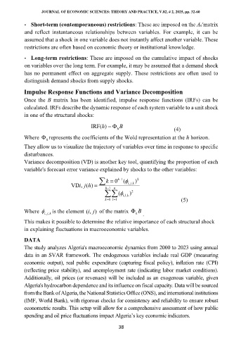
IRF( )h =  B
h (4)
Where  represents the coefficients of the Wold representation at the h horizon.
h
They allow us to visualize the trajectory of variables over time in response to specific
disturbances.
Variance decomposition (VD) is another key tool, quantifying the proportion of each
variable's forecast error variance explained by shocks to the other variables:

 k = 0 ( ) 2
h−
1
VD , ( )i j h = h− 1 n i , ,j k
  ( , ,l k ) 2
i
k= 0 l= 1 (5)

Where  i , ,j k is the element ( , )i j of the matrix  k B

.
This makes it possible to determine the relative importance of each structural shock
in explaining fluctuations in macroeconomic variables.

DATA
The study analyzes Algeria's macroeconomic dynamics from 2000 to 2023 using annual
data in an SVAR framework. The endogenous variables include real GDP (measuring
economic output), real public expenditure (capturing fiscal policy), inflation rate (CPI)
(reflecting price stability), and unemployment rate (indicating labor market conditions).
Additionally, oil prices (or revenues) will be included as an exogenous variable, given
Algeria's hydrocarbon dependence and its influence on fiscal capacity. Data will be sourced
from the Bank of Algeria, the National Statistics Office (ONS), and international institutions
(IMF, World Bank), with rigorous checks for consistency and reliability to ensure robust
econometric results. This setup will allow for a comprehensive assessment of how public
spending and oil price fluctuations impact Algeria’s key economic indicators.

38