Page 34 - Azerbaijan State University of Economics

3. Fuad Selamzade: Measurement of the Efficiency of Azerbaijan Region Hotel
4. Organization: Window Analysis and Malmquist Index

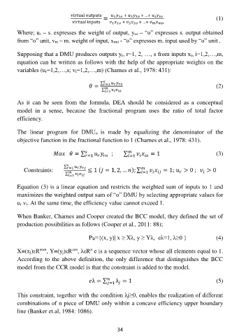
virtual outputs = 1 1 + 2 2 + ...+ (1)
virtual inputs 1 1 + 2 2 + ...+

Where; us – s. expresses the weight of output, yso – “o” expresses s. output obtained
from “o” unit, vm – m. weight of input, xmo - “o” expresses m. input used by “o” unit .

Supposing that a DMU produces outputs yr, r=1, 2, …, s from inputs xi, i=1,2,…,m,
equation can be written as follows with the help of the appropriate weights on the
variables (ur=1,2,…,s; vi=1,2,…,m) (Charnes et al., 1978: 431):

= ∑ =1 (2)
∑
=1

As it can be seen from the formula, DEA should be considered as a conceptual
model in a sense, because the fractional program uses the ratio of total factor
efficiency.

The linear program for DMUo is made by equalizing the denominator of the
objective function in the fractional function to 1 (Charnes et al., 1978: 431).

= ∑ ; ∑ = 1 (3)

=1
=1

∑ =1
Constraints: ≤ 1 ( = 1, 2, … ); ∑ = 1; > 0 ; > 0
∑ =1
=1

Equation (3) is a linear equation and restricts the weighted sum of inputs to 1 and
maximizes the weighted output sum of “o” DMU by selecting appropriate values for
ur vi. At the same time, the efficiency value cannot exceed 1.

When Banker, Charnes and Cooper created the BCC model, they defined the set of
production possibilities as follows (Cooper et al., 2011: 88);

PB={(x, y)| x ≥ Xλ, y ≥ Yλ, eλ=1, λ≥0 } (4)

sxn
n
X=(xj)εR mxn , Y=(yj)εR , λεR e is a sequence vector whose all elements equal to 1.
According to the above definition, the only difference that distinguishes the BCC
model from the CCR model is that the constraint is added to the model.

λ = ∑ λ = 1 (5)

=1

This constraint, together with the condition λj≥0, enables the realization of different
combinations of n piece of DMU only within a concave efficiency upper boundary
line (Banker et.al, 1984: 1086).

34