Page 13 - Azerbaijan State University of Economics

Yadulla Hasanli, Nazim Hajiyev, Gunay Rahimli:Distribution and Analysis of Admission
Scores (In the Case of Azerbaijan

As can be seen χ 2 =391.7. As the number of intervals k=10, the number of

parameters of the distribution s=2, the value of the degree of freedom r=k-1-s=7. At
this price of the degree of freedom, χ2(0,05;7)=14.07-dir. Thus, because inequality
of χ 2 < χ2-critic is not true in this case, we reject the hypothesis that scores

distributied normally.

Now based on table 2, let’s check whether the scores of azerbaijan section’s
applicants for the 1st group exam in the schooling year of 2017/2018 are subject to
exponential distribution. For this, we will make the table 5.

Since the mathematical expectation of a random variable in exponential distribution
is E(x)=1/ , to find , we can use the following formula: = 1/ ̅.

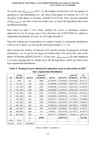
Here, because the number of intervals k=12 and the number of parameters of tested
distribution s=1, we get for the degree of freedom that r=10, and in this value of the

degree of freedom χ2(0,05;10)=18,31. In this case, χ 2 < χ2-critic inequality

is not true meaning that we should reject the H0 hypothesis which says that scores
have exponential distribution.

Table 5: Testing if scores obtained in admission exam to universities in 2017
have exponential distribution
group observed expected (O-
No interval up to b frequency p(x<a) p(a<x<b) frequency E)^2/E
1 0-60 60 5906 0.2549294 0.2549294 6523.6438 58.47712
2 61-120 120 4210 0.4448698 0.1899404 4860.5751 87.07775
3 121-180 180 3495 0.5863888 0.141519 3621.4715 4.416725
4 181-240 240 2980 0.6918305 0.1054417 2698.2519 29.41979
5 241-300 300 2424 0.770392 0.0785615 2010.3881 85.09541
6 301-360 360 2008 0.8289258 0.0585338 1497.881 173.7263
7 361-420 420 1494 0.8725377 0.0436118 1116.0271 128.0108
8 421-480 480 1045 0.9050316 0.0324939 831.51895 54.80832
9 481-540 540 832 0.9292418 0.0242103 619.54031 72.85905
10 541-600 600 600 0.9472802 0.0180383 461.60126 41.49515
11 601-660 660 419 0.96072 0.0134398 343.92552 16.38779
12 661-700 700 177 0.9677173 0.0069973 179.06112 0.023725
n= 25590 0.9677173 751.798
mean st.dev
203.89 162.55 0.0049046

Source: authors’ calculations

13