Page 12 - Azerbaijan State University of Economics

THE JOURNAL OF ECONOMIC SCIENCES: THEORY AND PRACTICE, V.78, # 2, 2021, pp. 4-16

The main disadvantage of the moment coefficient of asymmetry is that its value is
very sensitive to the sharp difference of any certain value of the variable in the
collection. The structural coefficient of asymmetry characterizes the asymmetry in
the central part. Unlike the moment coefficient of asymmetry, any sharp difference
in the value of variables does not affect the value of this coefficient. In practice, the
structural coefficient of asymmetry proposed by Karl Pearson is widely used.

x − mod
As pirson = 

In a variation sequence, if mode=median=mean, this means the sequence is symmetric.

If the mode of a variation sequence is less than mean, then the structural coefficient
of asymmetry becomes greater than 0, and thus the sequence is asymmetric to the
right. By contrast, if the mode of a sequence is grater than mean, in this case, the
structural coefficient of asymmetry becomes less than 0, which means the sequence
is asymmetric to the left.

RESULTS
Testing distributions of scores
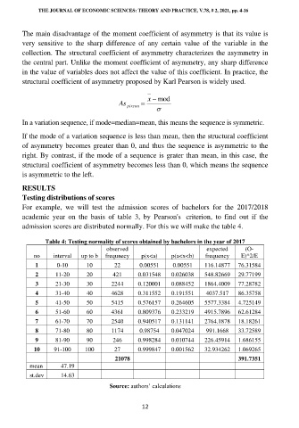
For example, we will test the admission scores of bachelors for the 2017/2018
academic year on the basis of table 3, by Pearson's criterion, to find out if the
admission scores are distributed normally. For this we will make the table 4.

Table 4: Testing normality of scores obtained by bachelors in the year of 2017
observed expected (O-
no interval up to b frequnecy p(x<a) p(a<x<b) frequency E)^2/E
1 0-10 10 22 0.00551 0.00551 116.14877 76.31584
2 11-20 20 421 0.031548 0.026038 548.82669 29.77199
3 21-30 30 2244 0.120001 0.088452 1864.4009 77.28782
4 31-40 40 4628 0.311552 0.191551 4037.517 86.35758
5 41-50 50 5415 0.576157 0.264605 5577.3384 4.725149
6 51-60 60 4361 0.809376 0.233219 4915.7896 62.61284
7 61-70 70 2540 0.940517 0.131141 2764.1878 18.18261
8 71-80 80 1174 0.98754 0.047024 991.1668 33.72589
9 81-90 90 246 0.998284 0.010744 226.45914 1.686155
10 91-100 100 27 0.999847 0.001562 32.934262 1.069265
21078 391.7351
mean 47.19
st.dev 14.63

Source: authors’ calculations

12