Page 11 - Azerbaijan State University of Economics

Aimene Farid, Bahi Nawel:Operational Risk Estimation Using the Value-at-Risk (VAR)
Method: Case Study of the External Bank of Algeria (EBA)

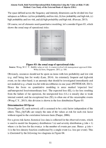
The space defined across the frequency and intensity dimensions can be divided into four
subspaces as follows: (a) low probability and low risk, (b) low probability and high risk, (c)
high probability and low risk, and (d) high probability and high risk. (Fawzan, 2015).

Of course, not all elements need quantitative modeling, let's consider Figure 03, which
shows the zonal map of operational risks:

Figure 03: the zonal map of operational risks
Source: Wong, M. C. Y.. Bubble value at risk: A countercyclical risk management approach John
Wiley & Sons, Singapore. 2013, p. 188.

Obviously, resources should not be spent on items with low probability and low risk
(e.g. staff being late for work) (Lam, 2014). An extremely frequent and high-risk
event, on the other hand, is an anomaly that should be investigated immediately and
not modeled (e.g. a bank was hit with ten robberies in one year) (PETITJEAN, 2013).
Hence the focus on quantitative modeling is areas marked 'expected loss'
and'unexpected loss/extraordinary loss'. The expected loss (EL) is the loss resulting
from the failure of the operation, the unexpected loss (UL) is usually due to weak
internal control, and the exceptional loss (XL) is often one of the catastrophic events
(Wong C.Y., 2013), this division is shown in the loss distribution Figure 03.

Determination Of Opvar
Given Figure 02, each network cell is assumed to be a risk factor independent of the
others. Thus, OpVaRs are simply the sum of the values at risk for each risk factor
without regard to the correlation between them (Panjer, 2006).

For a given risk factor, historical loss data is collected for the observed events, which
is used to model the frequency distribution f (n) and severity distribution g (x|n = 1)
where x is the loss for the event,n is the number of events per year. Hence g (x|n =
1) is the loss density function conditioned by a single event (i.e. loss per event). This
is illustrated by the following two diagrams in Figure 04.

11