Page 32 - Azerbaijan State University of Economics

THE JOURNAL OF ECONOMIC SCIENCES: THEORY AND PRACTICE, V.83, # 1, 2026, pp. 20-39

Regime 2 indicates periods of increased volatility being mostly a result of the global shocks
in energy and financial markets, while regime 1 indicates periods of relative market calm.
The estimates provided in Table 3 provide an indication of how the market fluctuated
randomly during the sample period. The differences in the mean and variance for both stable
and volatile periods clarify the cyclical movements that underpin market behaviour.
• Regime 1 (Low Volatility): characterized by small conditional variance (σ =
0.011) and moderate positive stock returns (μ = 0.0078).
• Regime 2 (High Volatility): marked by negative returns (μ = −0.023) and
roughly threefold higher variance (σ = 0.029).

Crises tend to be more intense even though they are often shorter, the average duration of
crises is approximately 13 months, while stable periods are significantly longer, often
averaging close to 21 months. This finding aligns with Bildirici and Badur (2019), who
identified three regimes: low, moderate, and crisis, and Mokni (2020), who found the
same stability patterns between energy and stock markets. In summary, this result
suggests that financial stress may behave somewhat differently depending on the
situation, and in addition, it tends to create more stress over time. Volatility thus tends to
accumulate and remain high at times when uncertainty increases, until macroeconomic or
policy changes bring things into progressive equilibrium. Such prolonged volatility
highlights the benefits of nonlinear transition models over more static GARCH
frameworks, as noted by Engle (2002) and Hamilton (1996). As evidenced by the
occurrence of periods of high volatility coinciding with important global events such as
the Eurozone crisis in 2011, the sharp drop in oil prices in 2014, as well as the COVID-
19 outbreak in 2020 and the conflict in Ukraine in 2022, energy shocks continue to be
one of the main causes of financial turbulence. This close timing supports the stability of
the MS-VARX model results and thus shows how stable the relationship between energy
and financial markets is under different economic circumstances.
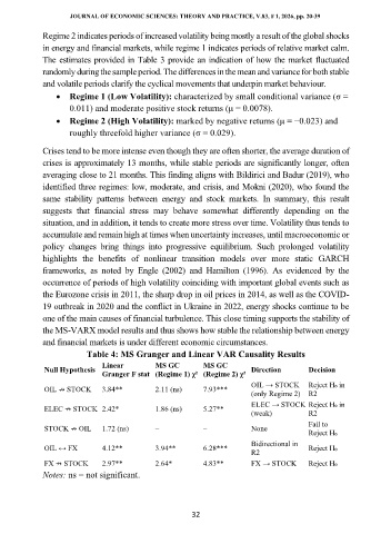
Table 4: MS Granger and Linear VAR Causality Results
Linear MS GC MS GC
Null Hypothesis Direction Decision
Granger F stat (Regime 1) χ² (Regime 2) χ²
OIL → STOCK Reject H₀ in
OIL ↛ STOCK 3.84** 2.11 (ns) 7.93***
(only Regime 2) R2
ELEC → STOCK Reject H₀ in
ELEC ↛ STOCK 2.42* 1.86 (ns) 5.27**
(weak) R2
Fail to
STOCK ↛ OIL 1.72 (ns) – – None
Reject H₀
Bidirectional in
OIL ↔ FX 4.12** 3.94** 6.28*** Reject H₀
R2
FX ↛ STOCK 2.97** 2.64* 4.83** FX → STOCK Reject H₀
Notes: ns = not significant.

32